Orthogonal Coordinates

It is convenient to use orthogonal coordinates, that is axes that are at right angles to each other. This permits the components along each axis to be described separately and independently. In this chapter we use Cartesian coordinates which are orthogonal. In the Cartesian system a vector is represented by its x and y components. When we draw the coordinate system (compare picture on the right), we use to lines drawn perpendicular to each other, that is to say with a 90^o angle between them. Conventionally, we label the horizontal axis with the letter "x" and the vertical axis with the letter "y".

Any point in this two-dimensional coordinate system can be represented by a vector, graphically represented by an arrow pointing from the origin of the coordinate system, x=0 and y=0, to the point in space.

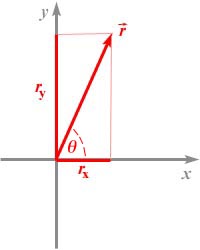
For example the position vector shown in the above figure has two components, a component along the x-axis, r_x, and a component along the y-axis, r_y. We can then symbolically express this vector by this pair of coordinates. We will use the notation shown here, a pair of numbers in brackets, separated by a comma:

= ( r_x , r_y )

If you now examine the above figure, you will note that r_x and r_y form a rectangle, which is divided into two right triangles by the vector . The sides of this triangle have lengths r_x and r_y, and the hypotenuse is the r-vector. The theorem of Pythagoras now tells us that:

|| = (r_x² + r_y²)^1/2

|| is the length of the vector, sometimes also simple denoted by r. So you see that you can figure out the length of the vector by knowing its x- and y-components.

You will also note in the figure that we have marked the angle between the x-axis and the r-vector by the symbol q (Greek letter theta), which we generally use to indicate angles.

More trigonometry will tell you that:

(This, by the way, is about as much trig as you will need for this entire chapter and probably for the entire course). This shows that we can also use the pair of numbers r, the length of the vector, and $\theta$, its angle relative to the x-axis, to describe the vector. In fact, this is the representation of the vector in polar coordinates, another orthogonal coordinate system.

Since you can construct the transformation from a representation of a vector in polar coordinates to one in Cartesian coordinates, it is also possible to construct the inverse transformation, from Cartesian to polar:

The upper of these two equations we already obtained above, and the lower one can then also be obtained with the aid of a little trigonometry.

The two yellow boxes on this page are the complete transformation equations between Cartesian and polar coordinates.

This page contains a great deal of new information, and you should really try to understand the concepts discussed here. Much of the difficulty that beginning physics students have comes from the lack of familiarity with the representations of vectors in different coordinate systems and the transformations between them.

© MultiMedia Physics, 1999